This is a Revised and Re-edited version dated Sep 2023 by A.E. for ChemEngmusings
The simulation model of a variable speed centrifugal compressor presented in the earlier post dated June 14, 2020 gives the development and formulation of a calculation model to describe the simulation of the performance curves and the shaft power requirements of an existing vsc-compressor. This simulation model consists of two sub-process models: an ideal, isentropic compression process and an energy / power loss process proceeding concurrently in the real, existing compressor machine. This simulation model fits on part of a single Excel worksheet.
In the current post, in this -improved and revised- version of Part II of “Simulating a Variable Speed Centrifugal Compressor”, we are presenting a further development of this simulation by extending it with ability to simulate the surge line and the choke line in performance diagrams. In addition a new sub-model is developed to describe and calculate the (shaft) power-losses i.e. the energetic losses not converted in a pressure rise but in an (additional) temperature rise. With this new Power-loss sub-model the total shaft power requirement can be calculated without the aid of an efficiency factor like as was presented previously in the earlier post (Part I).
This post is long, divided in ten sections. Sections “1)” and “2)” summarize the simulation model and its modeling approach and principles as given in Part I. The remainder of Sections “3)” to “9)” describe the new extensions and additions of the simulation model. In Section “10)” images of the simulation’s Excel worksheet are presented. These ten Sections are as follows:
‘1 Describing the principles behind the performance curves: a summary.
‘2 Fingerprinting the Characteristic Performance (Model Identification).
‘3 Describing the Surge Points and Surge Line in the Performance Diagram.
‘4 Describing the Choke Points and Choke Line.
‘5 Thoughts on the Shape of the Fingerprint Curve ‘ H*fp ‘
‘6 The Gas Power ‘Gad’ and the Unified ‘G*ad’ Curve.
‘7 The Shaft Power ‘Ps’ and the Adiabatic Efficiency Factor ‘Eta-ad’ .
‘8 Fingerprinting the Overall Power-Loss Process(es)
‘8.1 Determination of the losses during operation of compressor “vscCR-01” .
‘8.2 Pressure loss and Power Loss.
‘8.3 Characterizing the Overall Loss Processes.
‘8.4 Fingerprinting the Overall Loss Processes.
‘8.5 Predicting the Power Loss.
‘9 Predicting the Shaft Power in the Simulation of ‘vscCR-01”
’10 Upgraded and updated Simulation Excel Spreadsheet. The simulation consists of three parts on the same worksheet:
Part 1: Input data: Compressor Performance data ; Gas Quality data
Part 2 (A): Analyzing the Manufacturer’s data: calculation of Q* and H*
Part 2 (B) -1: ‘Fingerprinting’ the Performance Curves : H*fp
Part 2 (B) -2: Determination of the Surge – and Choke Points and Lines
Part 3: Simulation of Compressor “vscCR-01” including inter- and extrapolated speeds (7800 and 8800 rpm); the calculation of Discharge Pressure ; Pressure Ratio; Adiabatic Head; Gas Power; Power-Loss; Required (total) Shaft Power; images of the worksheet Part 2 and Part 3 are shown.
A pdf version of this entire post is given here: https://mychemengmusings.files.wordpress.com/2023/09/part-ii-revisit-and-edit-31aug23-simulating-an-existing-variable-speed-centrifugal-compressor-4-pdf-publ-revised-final.pdf
1) Describing the principles behind the performance curves: a summary
We have seen earlier that the performance of a compressor is often presented by the manufacturer in a graphical way through the ‘mapping’ of how the pressure ratio of discharge over suction absolute pressure varies with volumetric suction flow rate for a number of compressor speeds. Alternatively the absolute discharge pressure for a given suction pressure can be ‘mapped’ for various speeds. In addition the shaft power required to run the compressor under the conditions shown on the map is given. See earlier Charts for the particular existing compressor “vscCR-01” under study.
A simulation of the performance of a compressor in an excel spreadsheet is not and should not simply be a mathematical formula(s) just capable of capturing these curves on the map through curve-fitting, regression etc. Such formula’s are ‘blind’, are devoid of ‘insight’ into the essential principles at work in a running compressor and hence ‘risky’ to use outside the strictly specified operating conditions and parameters for which the compressor performance map was drawn. Parameters such as speed of rotation, feed rate range, gas quality with its many included physical property factors etc.
For this reason we have in the previous ‘Part I’ discussed the principles of a centrifugal compressor and its essential characteristics:
===> a centrifugal compressor in essence is a volume moving machine where the rotor design (impeller diameter, width , shape), in conjunction with gas quality, determines the gas volume moved per rotation.
===> a centrifugal compressor is a head producing machine as the turning rotor causes the gas to exit the impeller’s perimeter at high velocities creating “velocity head” that in the static part of the machine is converted into “pressure head”. (you could say “Bernoulli in operation”)
The volume of gas ‘moved’ by an impeller is determined by the fixed geometry of the impeller (diameter, width of ‘flow-channels’, number and shape of blades), the number of rotations per unit of time, the nature of the gas and how this gas flows, its ‘flow-pattern’, through the impeller.
Q1 = f * Qimp * S in which ‘Qimp’ is the volume the impeller can move per rotation which is fixed as per the geometric design of the impeller, ‘S’ is the speed of rotation, ‘f ‘ is the factor characterizing the flow pattern and ‘Q1’ is the resulting suction volume flow rate.
Thus we can write : Q1 / ( Qimp * S ) = f = nearly constant!
Note : Let us check the SI dimensions of the expression :
Q1 (m3/s) = f ( — ) * Qimp ( m3/rev) * S (rev/s ) : and hence ‘ f ’ is dimensionless.
Other units are commonly used to obtain more easily ’handled’ numbers like rpm, like Q1 in m3/hour and ‘S’ in rev/min or rpm. When these are used in this equation it means that we have to introduce additional constants to keep the equation whole and numerically consistent!
The ‘head’ producing capability of the compressor also roots in the geometric/mechanical design of the rotor and stator, the impeller(s) in particular. We have chosen to model the compressor as performing an adiabatic compression of a real gas. The impeller produces an adiabatic head (expressed in kJoule/kg)
‘Himp’ = 4 * Pi2 * S2 * D2 in which ‘S’ is the speed of rotation, and ‘D’ the impeller’s diameter. The volume moving capability is proportional to the speed of rotation, while the head is proportional to the square of the speed ! Higher speeds benefits higher heads stronger.
The total adiabatic head ‘Had ’ produced by the machine (impeller+diffuser) is influenced by the overall flow pattern through the machine (combined rotor and stator parts):
Had = hf * ‘Himp’ in which ‘hf ’ is the factor characterizing how the overall flow pattern is affecting the ‘production’ of adiabatic head ‘Had ’ generated by the machine
Had = * 4 * Pi2 * S2 * D2 and thus:
Had / (4 * Pi2 * S2 * D2 ) = hf and is nearly constant!
Note: Let us check the SI dimensions : Had (kJ/kg) = hf’ (–) * 4 pi * S^2 (rev/s)^2 * D^2 ( m2 ) ; remember that 1 Joule= 1Nm= 1kgm/s^2 * 1m then: Had ( m2/s^2 ) = hf (–) * 4 pi * (1 /s) ^2 * m2 and ‘hf ’ is dimensionless.
The unique performance of the existing machine is determined by its own geometrical configuration, its mechanical construction and its unique flow patterns established that are characterized by factors ‘ f ‘ and ‘ hf ’ .
These equations suggest that in order to describe the “head producing” and “volume moving” capability we would need the construction details of impeller’s, rotor, stator and more much more information to analyze the flow patterns in order to asses how they affect those two capabilities, i.e. the performance curves and power consumption!
However, we do not have such construction details that manufacturers are very reticent to share.
But wait ! At this point it’s good to keep in mind that we want to model the performance of our existing compressor, but do not want to step in the compressor designer’s shoes! We want to model the machine from a user’s perspective; we are looking from the outside in, and only want the variables we have control over to be (mathematically) described in terms of the basic principles at work in the operation of the compressor machine.
Therefore I have defined the following two variables to describe the performance curves of the existing compressor (see previous post Part I ):
Q* = Q1 / S * eps-h and H* = Had / (S/1000)2
in which Q* (say Q-star) and H* (H-star) are reduced variables with respect to the rotation speed ; ‘Q1’ is the suction volumetric flow rate ; ‘S’ the speed of rotation ; ‘Had’ is the adiabatic head developed at speed S and flow rate Q1 and ‘eps-h’ is defined as :
‘eps-h = Sqrt ( 2/ ( 1 + ( P2 * Z1 * T1) / (P1* Z2 * T2) ) )
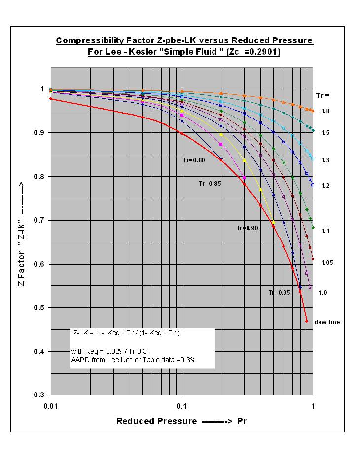
in which ‘P2’ is the compressor’s discharge pressure, ‘P1’ the suction absolute pressure, ‘Z1’ the compressibility factor of the gas at suction side, ‘Z2’ the compressibility factor of gas at discharge conditions and T1 and T2 the corresponding absolute temperatures. The Z factors, the gas compressibility factors, are calculated with the ‘Zv’ correlation published in earlier posts.
The ratio Q1/S, you could say, is the effective volume of inlet gas moved per rotation and ‘eps-h’ is the factor relating inlet gas density to the average gas density between inlet and outlet. The latter you could say accounts for the effect of speed on the average pressure across the machine and hence the average density of gas inside the machine!
The newly defined variable ‘ H* ‘ is calculated from the adiabatic head ‘Had’ that is in it’s turn is calculated with:
Had = Z1 * R/MW * T1 * k/(k-1) * [ (P2/P1)^( (k-1)/k) -1 ]
The adiabatic Gas Power follows from: Gad = Had * Fm
Please note that the calculation of the adiabatic head ‘Had’ in the above formula used in the simulation model includes gas compressibility factor Z1 based on the inlet condition conditions and not based on the average of in- and outlet conditions! For more on how these definitions were arrived at and used to make a “finger print” of our compressor machine see previous post with Part I.
2) Fingerprinting the Characteristic Performance (Model identification).
The fingerprint is the relationship describing the machine’s essential performance in terms of the reduced variables H* and Q*. By plotting all available performance data in terms of H* and Q*, I have found that the three (manufacturer provided) performance curves (speeds 5870, 7000 and 8330 rev/min) have coalesced into one single curve. This single relationship between H* and Q*, unique to our machine, has been captured by regression in a quadratic relationship between H* and Q*. It is this curve that defines the unique, fundamental relation between H* and Q*. This relationship I have called the ‘fingerprint’ with as symbol ‘H*fp’. This curve, as shown in the previous post, can be captured by a quadratic equation:
H*fp = A * (Q*)^2 + B * (Q*) + C ; for 0.258 =< Q* <= 0.438 ….…..(Eq.2-1)
With the help of this equation the compressor’s H – Q curves can be simulated. In other words with this fingerprint curve ‘H*fp’ a performance map for the original three speeds can be generated including those for interpolated or extrapolated speeds!
In the previous post we drew attention to the fact that all three surge points of the three original performance curves have now been “rolled” into one single point on the fingerprint ‘H*fp’ curve and that the (original) surge points and line can be reconstructed again from this single point by doing the reduction ‘transformation’ in reverse. In this Part II more details are given in the following sections on how the single surge point and single choke point can be transformed into surge and choke lines. Detailed equations for the reverse “unpacking” of the one single points on the H*fp curve into for surge and choke lines are given next. (For more details on the ‘fingerprinting’ see Part I).
In the above two sections 1) and 2) we have summarized the model development described in Part I. In the next sections of this Part II further extensions and developments of the simulation model are given.
3) Describing the Surge Points and Surge Line
No explicit information on the surge points or surge line in the performance map had been provided by the manufacturer. In the previous post, in Part I, I had assumed that the first point (lowest volume flow, highest pressure) of each of the three curves provided by the manufacturer was equal- or close to the surge point. In this Part II, I want to look closer into this. The fingerprint reduced head curve ‘H*fp’ variation with Q* has the shape of an inverted parabola (A is negative).
The operating points with lowest reduced flow rate on the curve are close to the “top” of the parabola while the slope of the curve gets increasingly smaller, i.e.the angle of the tangent line approaching zero degrees at the maximum of the curve.
Therefore I am defining the surge point as the point where the H*fp curve is at its maximum i.e. where the slope equals zero. The slopes of the H*fp curve can be found :
d (H*fp)/d(Q*) = 2 A * (Q*) + B ; hence at surge: 0 = 2A * (Q*surge) + B
===> Q*surge = – B/ 2A and H*fp-surge = – B^2 / 4A + C
These are the coordinates of the (reduced) surge point on the finger print performance curve. From these coordinates the surge points of any speed curve can be reconstructed as follows: first we need to calculate what the pressure ratio P2/P1 is under surge conditions for a given speed of rotation ‘S’ as follows :
(a) Had,surge = H*fp,surge * ( S/1000)^2
(b) (P2/P1),surge = [ Had,surge * MW / ( Z1 * R * T1 * k/(k-1) + 1 ] ^ (k/(k-1))
Note that the other points of the curve are calculated directly the H*fp fingerprint equation.
The actual suction volumetric flow ‘Q1’ at surge can be calculated from :
(c) Q1,surge = (Q*,surge) * S * 1/eps,surge
having the calculated (P2/P1),surge value, now the factor 1/eps,surge can be calculated as:
(d) 1/eps,surge = ( ½ + ½ * (P2/P1)^(1/k) * Z1/ Z2 )^0.5
in which ‘Z2’ can be calculated iteratively (simple substitution) as is done for the simulation calculations of other points on the curve. Note that the last equation (d) includes already the adiabatic temperature ‘T2’ calculation.
These calculations (a) to (d) have been implemented in the upgraded Centrifugal Compressor Simulation spread sheet. In Section 10 a copy of the worksheet Part 2 (B)-2 is shown.
Note: Having defined the surge point and determined its coordinates on the compressor’s “fingerprint” performance map (plotted in reduced variables H* and Q*) we can now describe the H*fp quadratic equation in an alternative way using these coordinates:
H*fp = H*surge – (A”) * (Q* – Q*surge )^2
in which A” = -1 * A ; and when inserting the numerical values of the surge coordinates we get:
H*fp = 0.92760 – 7.5914 * (Q* – 0.24 )^2
4) Describing the Choke Points and Choke Line
No explicit information on the choke points or choke line was divulged by the manufacturer either! What do we know about ‘Choke’ ? The word itself already is very suggestive, you choke when you are overwhelmed by food or drink and cannot swallow it any more. That happens to a centrifugal compressor too when at a given speed and operating point (discharge pressure, volume flow rate) you start to increase the feed rate to the machine more and more. As the feed rate increases the outlet pressure drops (following the curve). At a certain high feed rate the outlet pressure starts to drop more steeply while the ability to process the increases in feed rate diminishes strongly until the outlet pressure falls to a dramatically low value while the feed rate cannot be increased anymore: it appears as if the operation has run into a stone wall.
Why does this happen? An impeller increases the velocities of the gas flowing through it by the centrifugal forces acting on it. The velocities of the gas reach their highest value at the exit perimeter rim of the impeller. The compressor is designed for a given operating point of speed, feed rate and discharge pressure with the rotor and stator geometrically shaped to have their maximum energetic efficiency point, or in other words to have a minimum of energetic losses at that design operating speed and for that given gas quality. By more and more increasing the feed rate the internal gas velocities across the impellers consequently increase more too! The velocity increase is more prominent as the operating point moves along the curve towards lower outlet pressures and higher temperatures. When a point along the flow path inside the machine has reached locally (likely the exit of one of the impellers) a gas velocity approaching the speed of sound of the particular gas, the “sound barrier” is being reached. The velocity of sound cannot be exceeded! The choking point has been reached!
(as an aside here: it is interesting to note how tech- people view and see their equipment / devices they are working with: they ascribe ‘life’ to it, see it like a living thing! it can make surging, regurgitating sounds ; it can choke on what it is fed etc perhaps you can find more examples of similar sayings ?)
To be able to evaluate where our compressor’s operating point is with respect to the choke point or choke line we would need to look at the internal velocities, however without detailed info of the internal machine dimensions that is impossible. We can however calculate what the discharge internal volumetric flow rate Q2 is for a given operating point on the curve. Our model allows us to calculate the gas density Rho2 at discharge Pressure P2 and hence:
Q2 = Fmass/ Rho2 = Q1 * Rho1 /Rho2
When we calculate Q2 for all three curves provided by the manufacturer we can see an interesting picture emerge: for each of the three curves the first point indicates that Q2 equals about 0.25 m3/s, then for the next points along the curve Q2 gradually increases while the last points provided show the volume flow rates of the compressed gas Q2 are approaching a value of about 0.5 m3/s irrespective of speed and discharge pressure (P2) level generated. To be precise for the last point of the speed curve at 7000 rev/min we see Q2 reaches 0.50 m3/s ; for 8330 rev/min Q2 reaches 0.56 m3/s while for 5870 rev/min the last point (of only five) reaches 0.43 m3/s.
These observations all hint, in my mind, to the conclusion that all the last points on the manufacturer’s curves are approaching a limiting value for the Q2 volume flow rate. Without detailed construction data we cannot ascertain or estimate the corresponding highest velocities values, but we can nevertheless do an order of magnitude check using the apparently converging Q2 flow rate value of 0.56 m3/s and the fact that the speed of sound in propane at 20 Bar is around 250 m/s (see later post for this).
The last points provided by the manufacturer likely (I am speculating) are the nearest points closest to their choke points that can be safely operated.
Therefore for our modeling purposes I am defining the Choke point as the last point on the H*fp curve at that point the Q* value equals 0.440 (rounded value).
From this defining value of Q*,choke =0.440 we find H*fp ,choke = 0.62389 . This value simply follows from calculation with the fingerprint equation H*fp (section 2).
These two values are the coordinates of the (reduced) Choke Point. From these coordinates the choke points of any speed curve can be reconstructed (and hence the Choke Line) in the same way as described in Section 3 for the Surge Point and Line with equations (a) to (d).
5) Thoughts on the Shape and Slope of the Finger Print ‘H*fp’ Curve
In the above discussion of the surge point and the choke point I have referred to the shape and the slope of the performance curves and in particular to the essential, reduced performance curve that I have called the “fingerprint” curve “H*fp ”. For example we have defined the surge point as the point where the H*fp curve reaches its maximum value i.e. when the slope of the tangent line to the curve approaches a value of zero, i.e. the tangent line running parallel to the Q* axis ( its angle = 0). It is interesting to note that the slope and angle of the tangent line in the (manufacture’s given) first point on the curve has an angle of minus 16 degrees. The initial part of the curve between the newly defined surge point and this first point is hence rather ‘flat’. From a control point of view it means that a small change in the reduced head H* is associated with a much larger change in Q* value and therefore small disturbances in head caused by small, frequent variations in rotation, pressures, temperatures, gas quality – process and equipment noise – cause much larger changes in Q* and hence the compressor operating in this part of the curve cannot “find“ and “settle” on a single, fixed operating point causing instabilities in the operation and these maybe the precursors to surging conditions. (see Chart given below).
In the discussion of the choke point we referred to the fact that when this point is reached during the operation of a ‘campaign’ (or a test) of ‘pushing’ the feed rate as high as possible, the outlet pressure drops, the performance curve sharply bends into a line at a 90 degree angle to the flow axis (the stone wall).
It is interesting therefore to look closer at the shape and slope of the performance curve. The performance maps as presented in previous Charts of Part I can be somewhat deceiving as they look rather “flat” because of the different scales at which they are plotted! Let us examine how the slope of the ‘fingerprint curve H*fp’ varies with Q* . The ‘slope’ = 2A * (Q*) + B and the angle of the tangent line in degrees = 180/pi * ATAN (slope).
In the following Chart I have plotted the H*fp equation versus Q* at equal scales so as to have a proper impression of the steepness of the performance curve. In addition also the Surge – and Choke points (as defined) are shown together with a number points marked with the angles of their tangent lines.

Diagram-1 Fingerprint H*fp versus reduced Inlet Volumetric Flow rate Q* drawn at equal scales.
The Diagram shows for three of the 12 points the angles of their tangent lines, whereas on the right hand side of the Chart the coordinates of surge – and choke points are given.
Note that the fingerprint performance curve at our defined choke point is sloped downwards at angle of nearly -72 degrees! That fact also has implications for controlling the compressor operation. Is the initial part of the curve close to the surge point nearly ‘flat’, for the end part we find the curve gets rather steep where small variations (this time ) in Q* have a much larger effect on H* and hence instabilities here also play a larger role in the operation.
Furthermore note also : To study the effect of making a potential change in the whole suction and discharge piping system of which the compressor is part, for example to save on energy consumption by the compressor, the ”system pressure loss- or resistance curve” needs to be drawn and examined in this reduced performance diagram. In particular it is the intersection of these two curves that determine the operating point of the compressor. It is the angle between these two curves that needs to be looked at vis a vis the controllability.
6) The GasPower ‘Gad’ and the unified ‘G*ad’ ‘fingerprint curve’.
The Adiabatic Gas Power ‘Gad’ required to perform the adiabatic compression of the gas in our machine follows straight forwardly from the model calculations as summarized in Section 1 and further detailed in Part I in the previous post!
The Adiabatic Gas Power ‘Gad’ at a given operating point on the curve follows directly from the adiabatic compression calculations: it is simply the product of the mass flow rate and the adiabatic head ‘Had’
Gad = Had * Fm ( kW = kJ / kg * kg / s ) …………………………(Eq.6-1)
We can express this relation also in terms of the two new variables, the reduced head H* and the reduced inlet volume flow rate Q* that we introduced to find the machine’s fingerprint relation H*fp, which is the essential speed independent relation between the adiabatic head H* and the inlet volume flow Q* for our existing compressor machine under study.
Remembering that we defined as H* = Had / (S/1000)^2 and as Q* = Q1 / S * eps-h and that the mass flow is Fm = Rho1 * Q1 ; we can re write Eq.6-1 as :
Gad = (H*) * (S/1000)^2 * Rho1 * (Q*) * S / eps-h ………………..(Eq.6-1a)
Note that in our definitions of H* and Q* we have kept the following units:
Had is expressed in kJ/kg , Q1 in m3/hour and S in rev/min and Rho1 in kg/m3 in order to obtain values for H* and Q* between 0 and 1 .
Hence to keep the units of the right hand side of the equation Eq.6.1-a consistent with the left hand side (kWatt) and to avoid dealing with large numbers like S^3 , additional constants have to be introduced and next after rearranging the expression becomes:
Gad = (H*) * (Q*) * (S/1000)^3 * 1000/3600 * Rho1 /eps-h …………(Eq.6-2)
This equation relates the adiabatic Gas Power, Gad, for a given operating point with the specific values of the reduced adiabatic head H* and the reduced volume flow Q* for that particular operating point.
By Defining G*ad (say Gad-star) as the reduced Adiabatic Gas Power as follows:
G*ad = Gad / (S/1000)^3 /Rho1 * 3.6 * eps-h ……………………….(Eq.6-3)
We can simply write the relationship between adiabatic gas power, the head and flow in terms of three reduced variables in a form analogous to the original equation Eq.6-1 as follows:
G*ad = (H*) * (Q*) ……………………………………………………….(Eq.6-4)
This equation is also valid for any operating point!
We have found that for this compressor there is an essential , speed independent relation we called the “fingerprint reduced adiabatic head” with as symbol: ‘H*fp’ characterizing our compressor:
H*fp = A * (Q*)^2 + B * (Q*) + C …………………………See (Eq.2-1)
Substituting H*fp in Eq.6-4 gives us the essential , speed independent , reduced adiabatic gaspower fingerprint relation that we will symbolize with ‘G*adfp’ and can bewritten as:
G*adfp = H*fp * (Q*) …………………………………………………….(Eq.6-5)
Alternatively as
G*adfp = [ A*(Q*)^2 + B*(Q*) + C ] * (Q*) …………………………… ..(Eq.65a)
From this we learn that Gad is a function of the third power of the speed and the third power in Q* (as polynomial) as well !
We have seen that the H*fp expression alternatively can be written as:
H*fp = H*surge – (A”) * (Q* – Q*surge )^2
In which ‘H*surge’ and ‘Q*surge’ are the coordinates of the surge point in the H* – Q* diagram. With this alternate H*fp expression we can also write this relation in an equivalent but more insightful form:
G*ad = [ H*surge – (A”) * (Q*-Q*surge)^2 ] * (Q*)
With these relations between the three reduced variables, G*ad, H* and Q* we have extended the H*fp equation into the reduced adiabatic Gas Power relationship. The H*fp equation is based on a regression correlation of H* – Q* values obtained from the adiabatic compression calculations (see ‘Part I’ in previous post).
Hence the G*ad relation is the unique fingerprint of the adiabatic gas power requirement of our machine to obtain the achieved compression performance.
The values of Gad follow directly from the Had and Fm values generated by the model
and thus if we plot the G*ad relation versus Q* and co-plot the directly calculated Gad values for all three speeds for all 25 points and they should all fall at – or very close to the G*ad fingerprint curve ! See next Diagram.

Diagram-2 The reduced Adiabatic Gas Power “ G*ad ” versus the reduced Inlet Volumetric Flow rate Q*.
To summarize : in this section 6 I have extended the adiabatic compression sub-model by defining the reduced Gas power G*ad. This reduced variable relates directly to the reduced Head ‘H*’ and the reduced flow rate ‘Q*’.
7) The Shaft Power ‘Ps’ and the Adiabatic Efficiency Factor ‘Eta-ad’.
The shaft power to drive the compressor is in part consumed by the production of increased outlet pressures, being the adiabatic gas power Gad part, and the remainder by “energetic losses” incurred through concurrent loss processes.
Now we do have a theory to describe the adiabatic gas power part, as used in our model, there is however no straightforward single piece of theory to describe the “loss” part.
There are many contributors adding to – and factoring into these energetic losses in their totality. I will come back to these in the next section 8-1.
The Gas Power required to perform the adiabatic compression of the flowing gas in our machine follows straight forwardly from the model calculations as already summarized in Section 1 and further detailed in Part I in the previous post and further “extended” in section 6 of this PART II.
In our earlier analysis of the existing compressor’s performance as given in Part I we have related our theoretical calculation of ‘Gad’ to the actual required total shaft power, data that the manufacturer provided, by means of the Adiabatic Efficiency Factor “Eta-ad”. Once this factor is known the shaft power can be calculated as:
Ps = Gad / Eta-ad. (units: kW = kW / (–) ) …………………..…………(Eq.7-1)
‘Eta-ad’ is here the sole factor, the key to arriving at the total required shaft power to drive the compressor. This factor in one single number wraps the gas power and all the contributing flow resistances and their corresponding power losses into a single number!
No single piece of theory exists, as far as I am aware of, to predict the extent of the sum-total of these losses, although through the decades over time empirical or semi-empirical correlations of contributing factors have been developed to be able to estimate a part of these losses. The capability to predict such losses is important in particular from the compressor designer’s perspective.
Therefore through ‘looking’ at the model‘s data and the manufacturers shaft power numbers, through trial and error I found , as described in Part I , a correlation for the adiabatic efficiency factor ‘Eta-ad’ and how it relates to the flow variable I had defined as ‘Q* ’ as follows:
Eta-ad * (S/1000)^0.39 / (Q1/S) = A * (Q*) + B ………………………(eq.7-2)
in which the constants are: A= – 8.4625 and B = 6.082
This correlation allows the total shaft power ‘Ps’ to be calculated from ‘Gad’ with an average percentage error of 0.67%!! Not bad! See Part I showing a Diagram where the predicted shaft power and the manufacturers quoted shaft power numbers are co-plotted to compare them in a visual way.
This “powerful” correlation I found, remarkable though it is, is only strictly valid for this compressor machine, the vscCR-01, to use as predictor! It is a correlation of connected variables that influence each other, however it does not reveal much insight into the scope and limitations of the application- and use of this equation. Therefore if you are going to apply this correlation in the simulation of your compressor beware and be cautious.
It is for this very reason that in this PART II, that I have taken a closer look, attempting to find other ways to calculate the total shaft power requirement ‘Ps’ by focusing directly on the power losses themselves in order to get a better ‘feel’ and more insight through developing a relationship for these losses with the operating parameters and variables of the compressor. This is dealt with in the next section 8.
8) Fingerprinting the Overall Power – Loss Process(es)
8.1 Determination of the losses during operation of compressor “vscCR-01” .
Energetic losses in a compressor are due to ‘flow resistances’ present along the path-way a gas follows through the machine. Both the stator and the rotor part contribute to the losses. The impeller, it’s geometric shaping and dimensioning, plays a major role in the generation of losses. Study and research over the decades have identified various types of resistances contributing to the overall loss of power experienced. Losses such as “incidence loss”, impeller “skin friction losses” and many more! Such detailed account of loss factors and how to describe these and how to calculate these in detail are of prominent importance to compressor designers and manufacturers, witness the large amount of studies published devoted to this subject.
From our perspective the question is can we find a description of how the overall, the sum-total of all these loss factors, relates to the adiabatic gas power production in vscCR-1 and how it figures into the total shaft power requirement to drive the compressor.
In PART I we have described the approach taken to formulate a Model of this variable speed compressor vscCR01. The Simulation Model conceptualizes the variable speed compressor, shown in the block diagram 4 of Part I, as consisting of two processes occurring side by side: the adiabatic compression process and a “loss process”. This implies that the total shaft power is the sum of the gas power plus the power consumption by the ‘loss processes. The ‘Power Loss’ part hence can be directly calculated from the Manufacturer’s quoted shaft power ‘Ps’ (in kW) and the adiabatic gas power ‘Gad’ calculated with our adiabatic compression sub-model:
Ps,loss = Ps – Gad (all expressed in kW) ………..………………..(Eq.8-1)
Let us picture how these losses look by calculating for each of the three speeds the power losses and plot these against the suction volumetric flow rate: (click on picture to enlarge):

Diagram-3 The Power Loss ‘Ps,loss’ versus inlet Volumetric Flow rate ‘Q1’
The graph shows the higher the inlet flow rate for a given speed the steeper the rise in ‘Ps,loss’ ; i.e. in the part of the total shaft power that is not converted into a pressure rise but in a temperature rise! The highest speed curve shows the power loss rise rather dramatically! One thing worth noting in the graph is that the first part of each loss curve is rather flat! I will come back to the significance of this observation in a future post (effect of combined incidence and friction losses)!
Next let us focus on the 8330 rev/min speed curve in detail and see how it’s (total) shaft power, adiabatic gas power and the power loss behave when shown in one single graph (click on picture to enlarge):

Diagram-4 Compressor Shaft Power , Adiabatic Gas Power and Power Loss versus Inlet Volumetric Flow rate ‘Q1’.
The total shaft power, not unexpectedly, increases with increasing volume flow rate. The curves for the two concurrent processes: the adiabatic compression and the power loss process(es) show a very interesting pattern: their curves look like they are each other’s mirror image! And that is no coincidence as I will show later. Similar pictures are found for the two other speeds.
‘ 8.2 Pressure Loss and Power Loss
Therefore let us examine closer the losses at a constant speed of rotation. Power added to the shaft that is “lost” towards the ultimate purpose of the machine to raise the pressure of the gas exit stream, is a loss of pressure (increase) not achieved. The term “pressure losses” is a familiar one in the context of hydraulic flow systems and engineering science. Thus let us start with the most well known and used semi-empirical relation to describe pressure losses across a ‘conduit’ carrying a fluid flow to aid in analyzing the “overall’ losses:
Delta P = K * ½ * Rho * v ^2 ………………………………………..(Eq.8-2)
In which ‘Delta P’ is the pressure difference along the conduit and in which “K” is a factor characterizing the total resistance to flow through the conduit. ‘Rho’ is the fluid density and ‘v’ the average velocity. (Note f = Fanning friction factor and 4f the Moody friction factor for pipe flow; see principles described in a future post).
In our case ‘P2’ and ‘P1’ are the compressor discharge and inlet pressures respectively; the density ‘Rho’ is not constant as we are dealing with a compressible gas flow and as we have elaborated in section 3.2 and 3.3 of PART I, equation eq.8-2 takes the following form:
Delta P = K * ½ * 1/ Rhoavg * (Fm/ Ac)^2 ; or:
P2 – P1 = DeltaP = K / Ac^2 * ½ * Q1^2 * Rho1^2 / Rhoavg
in which ‘Ac’ is the average cross-sectional area and ‘Rho1’ is the gas density at the inlet; ‘Rhoavg’ is the (algebraic) average density inside the machine over in- and outlet and ‘Fm’ the mass flow rate and Q1 is the inlet volumetric flow rate.
Note 1: the dimension of Pressure [P1] and [P2] = N/m^2 or Nm / m^3.
Note 2: the pressure difference here has a negative sign see comments in future post.
If we divide both sides by ‘Rho1’ the left hand side obtains the dimension of Nm /kg or Joule/kg and we get:
(P2 – P1) /Rho1 = K / Ac^2 * ½ * Q1^2 * Rho1 /Rhoavg
In PART I we have defined the ratio Rho1 /Rhoavg as “eps-h^2” and thus:
(P2-P1) /Rho1 = K / Ac^2 * ½ * (Q1*eps-h)^2 ……………………………(Eq.8-3)
The power required to drive the flow of fluid through the resistance formed by the shape and size of the conduit, we find by multiplying with the mass flow ‘Fm’ in kg/s
(P2-P1)/Rho1 * Fm = K / Ac^2 * ½ * ( Q1* eps-h )^2 * Fm
The left hand side is the power (loss) in Watts.
By analogy we are now applying this relation to the overall power losses generated by all the resistances posed to the gas flowing through the internals of the compressor or more precisely said: while being driven by the centrifugal forces via the diffuser to the discharge. Granted, the “conduit”, the ‘flow-channel’ through which the gas is passing from inlet to discharge is of complex form and shape for sure! Nevertheless, we equate the overall power loss “Ps, loss” in the compressor with the right hand side of the equation:
Ps,loss = K / Ac^2 * ½ * ( Q1*eps-h )^2 * Fm ……………………………..(Eq.8-4)
Note1: Let us check dimensions when expressing in SI units: Watt = J/sec = (—) / m2 * (m3/sec)^2 * kg/sec kgm/sec^2
Note2: “Ps” is the total shaft power to operate the compressor; Ps,loss the part of Ps consumed by overcoming resistances to flow and converted into heat. The factor ‘K’ is the sum-total of all contributing resistance factors and is applied here analogous to the ‘accounting’ of resistances as is done in the ‘theory and practice’ of hydraulic systems, for instance liquids flowing through a piping system, consisting of a straight long pipe fitted with a series of different “fittings” like pipe bends, pipe diameter changes, valves, orifices and so on. The additional flow resistances that these fittings add to the total have been (semi-) empirically measured and determined and can be added to the value of ‘K’. An interesting piece of information is the fact that in hydraulic systems the factor ‘K’ is not constant, even after the accounting for the configuration of the conduit carrying the flow, but is still dependent on the mass flow rate. For example for turbulent flow through smooth long circular pipes H. Blasius found that the “friction factor” depends on the Reynolds number as follows:
“friction factor” = Constant / Re^1/4 for turbulent flow 4000 < Re < 10^5
Noteworthy is the inverse relation ship with flow rate as indicated by the inverse Reynolds number, meaning the higher the flow rate the lower the friction factor!
In the further development of equation 8-4 we should keep in mind that the factor ‘K’ itself may be a function of flow rate (volume or mass or reduced volume flow rate Q*).
‘8.3 Characterizing the Overall Loss Process(es)
For centrifugal compressors the different resistances adding to the overall resistance to flow are many and complex and have been studied and used in the design of compressors in order to minimize energy losses at the required – design – operating point. As said we will keep to the user’s perspective in our analysis not the designer’s perspective and try not ‘zoom’ too much into the detailed individual loss contributors but keep the focus on the overall losses.
The adiabatic compression theoretical part of the Compressor Simulation Model calculates the adiabatic head, equal to the difference in enthalpy of the gas between inlet and discharge, at constant entropy. The adiabatic head ‘Had’ is expressed, like enthalpy, in kiloJoule per kilogram of gas.
To analyze the loss process and fingerprint the essential, characteristic of the (overall) loss process we should therefore similarly look at the power loss per kg of gas!
Let us see if and how the last diagram (Diagram-4) changes if we now plot ‘Had’ together with ‘Ps,loss’ and ‘Ps’ the latter both now expressed on a ‘kJ/kg’ basis by calculation of ‘Ps,loss’ divided by the mass flow rate ‘Fm’ and do the same for ‘Ps’. Plotting these three versus mass flow rate ‘Fm’ for the highest speed of 8330 rpm and as shown in the next Diagram-5 (click on Chart to enlarge):

Diagram-5 ‘Ps,loss/ Fm’ and ‘Had’ and ‘Ps/ Fm’ versus Mass Flow rate ‘Fm’.
Looking at this graph immediately the steady, nearly linear decrease of the shaft power divided by the mass flow rate jumps out! But just as striking is the fact that the “mirroring” of the adiabatic head curve with the curve of the power loss over mass flow rate has become even more pronounced and clearer!
‘8.4 New reduced variable “ H*,loss ” + Fingerprinting the Overall Loss Process.
In the following we are searching, with the help of the last equation Eq.8-4, for insight into how the losses relate to the operating conditions of flow, speed and pressure. Can we probe into these losses (without having construction details of internals) by analyzing the operating data in the same manner as done for the performance curves and adiabatic gas power modeling? And the answer is yes! How? By trying to find the unique relationship describing the losses, a unified, “fingerprint” relation for the overall resistance factor “K” that according to Eq.8-4 lies at the core of the overall loss phenomena exhibited by this compressor.
Let’s express the power loss in kJ/kg by taking Eq.8-4 and dividing both sides by the mass flow rate ‘Fm’ and we get:
Ps,loss / Fm = K / Ac^2 * ½ * ( Q1 * eps-h)^2
Note: the dimension of the left hand side: kW /(kg/s) = kJ/kg.
If in analogy with our definition of the reduced adiabatic head H* = Had /(S/1000)^2 , with units in kJ/kg/ (rev/min)^2 , we again divide both sides but this time by (S/1000)^2 we get:
Ps,loss / Fm / (S/1000)^2 = K / Ac^2 * ½ * ( Q1 * eps-h )^2 / (S/1000)^2
and remembering and including the definition of Q* and rearranging we get :
Ps,loss / Fm / (S/1000)^2 =1E+6 * K / Ac^2 * ½ * ( Q* )^2 ………….…..(Eq.8-5)
On the left hand side we have the energetic losses expressed as a new reduced variable with on the right hand side an expression involving the reduced volume flow rate Q*.
Therefore I am defining the left hand side of Eq.8-5 as “H*loss” . Thus we can write:
H*loss = Ps,loss/Fm/(S/1000)^2 = 1E+6 * K / Ac^2 * ½ * (Q*)^2 ………(Eq.8-6)
The question now is does this equation describe the power losses shown in the first Diagram of ‘Ps,loss’ versus inlet volumetric flow rate Q1? If indeed the factor ‘K’ , the overall resistance factor to flow, is a constant then the answer should be yes, because we have here the essential relationship of energetic losses with the square of the reduced flow rate.
This means that if for all three speeds and all points we plot the left hand side, ‘H*loss’ versus Q* we should get all data points to ‘coalesce’ into a single line!
Therefore I have plotted the left hand side for all 25 data points against Q* and found, as you can see in the next Diagram-6, that the points show some ‘aggregation’ into a sort of band but not as a clear single line as the next Diagram shows:

Diagram-6 ‘Ps,loss/Fm/(S/1000)^2’ versus reduced Inlet Volume Flow rate ‘Q* ’ for 3 speeds.
The points nevertheless show a definite trend: the higher the reduced flow rate the lower the value of the resistance factor ‘K’. When performing a regression on this scattered band only low r^2 correlation values are obtained (see Diagram-6).
Next, then tried plotting the ‘K’ values versus the inlet volumetric flow ‘Q1’ and following this plot next I made yet another plot against the mass flow rate. Both these plots (not shown here) displayed three distinctly separate lines for each of the speeds, with no aggregation, no banding, no coalescing of points into a single line, no unification. Now what to do?
Then remembering the possibility of ‘K’ not being a true constant! Furthermore remembering that even for a simple geometric shape like a straight circular pipe the overall resistance factor ‘K’ is not constant and still shows some dependency on mass flow rate. Therefore, with the “complex form and shape” of the gas flow channel (an understatement) present in our compressor we should check how ‘K’ in equation Eq.8-6 behaves! So let us see if indeed ‘K’ varies with ‘Q*’ and if so how. In the next Diagram I am plotting ‘K’ versus Q*. With ‘K’ based on Eq.8-6 as:
K = H*loss /(Q*)^2 = Ps,loss / Fm / (S/1000)^2 / (Q*)^2 * 2E-6 * Ac^2 ….(Eq.8-7)
Ignoring for the moment the factors 1E-6 * 2 * Ac^2 as truly constant then calculating the values of ‘K’ for all 25 data points (three speeds) and plotting these against ‘Q*’. I found these points form a much narrower a band. Then next through trial and error I found that all data points could be found forming a single line if plotted against the following expression: “ 1/ (Q*) * eps-h^0.44 “ as the following graph shows:

Diagram-7 Fingerprinting the flow resistance K*fp for compressor ‘vscCR-01’.
This Diagram shows that the overall flow resistance factor ‘K’ characterizing compressor ‘vscCR-01’ is inversely related to the reduced flow rate Q*. In other words the higher the flow-rate through the compressor the lower the overall resistance factor becomes. And as we have seen before, this is not unlike the relationship in hydraulic systems like the one quoted except here the inverse relationship is much more pronounced. As shown in the Diagram-7 the resistance factor values plotted are very well described by the following quadratic equation:
overall resistance factor K = A * x^2 + B * x + C ……………………. (Eq.8-8)
in which x = 1/(Q*) * eps-h^0.44 ; and A = 2.2731 ; B = -8.2188 ; C = 9.4235
The bold symbol K is a re-definition of ‘K’ of Eq.8-7 to include the factor Ac, being the inverse of the cross sectional area averaged over the flow path, and the conversion factors related to the units employed in this equation: kilo Watts, mass-flow in kg/sec and speed in rev/min instead of Watt, kg/hr, rev/sec or radians/sec.
This quadratic relationship of K with Q* is the essential, overall resistance “fingerprint” function describing how the overall resistance posed to the gas flowing through the internals of the compressor during the operation of ‘vscCR01’ varies with the reduced inlet volume flow rate, while being independent of speed. I will refer to this relation of K (Q*) with the symbol “K*fp ” :
K*fp = A * (eps-h^0.44 / (Q*) )^2 + B * (eps-h^0.44 / (Q*) ) + C …..…. (Eq.8-9)
With the constants A, B and C as given before in Eq.8-8.
The reduced loss ‘H*loss’ of Eq.8-6 can now be compactly written in reduced variables as:
H*loss = (K*fp) * (Q*)^2 ……………………………………………….……..(Eq.8-10)
With the help of equation Eq.8-9 the power loss ‘Ps,loss’ then is calculated as:
Ps,loss = (K*fp) * (Q*)^2 * Fm * (S/1000)^2 ………………………………(Eq.8-11)
Note that ‘Ps,loss’ is in kW if ‘Fm’ is expressed in kg/sec and ‘S’ in rev/min).
With Eq. 8-11 and the resistance fingerprint Eq. 8-9 we should be able to predict the shaft power losses, i.e. that part of the shaft power not converted into a gas pressure rise but instead converted into a temperature rise !
‘8.5 Predicting the PowerLoss ‘Ps,loss’
Taking the combination of equations Eq.8-9 and Eq.8-11 and calculating the values for Ps,loss as function of Q*. This combination gives the following ‘working” equation :
P2,loss =(2.2731* X^2 -8.1128 * X +9.4235) * (Q*)^2 * (S/1000)^2 * Fm ..…(Eq.8-12)
In which “X” stands for eps-h^0.44 / (Q*)
The following Diagram shows these predicted power loss calculated values versus the corresponding inlet volume flowrate ‘Q1’ , together with the co-plotted power loss values directly calculated from the Manufacturer’s quoted shaft power minus the adiabatic Gas Power values. (click on chart to enlarge):

Diagram-8 Predicted Power Loss compared with Actuals for Compressor “vscCR-01”.
To be precise: the overall average percentage error between predicted and actual loss data were calculated to be equal to 1.4 % !
Worth noting are the alternate ways in which Eq.8-11 can be written:
Ps,loss / Fm = (K*fp)* (Q* )^2 * (S/1000)^2 ……………………………..(Eq.8-11a)
In this equation the term ‘Ps,loss/Fm’ can be interpreted as the enthalpy difference ‘DeltaH’ associated with the energy being converted into heat as a result of loss processes during compressor operation!
DeltaH,loss / (S/1000)^2 = K * (Q* )^2 ……………………………….……(Eq.8-11b)
Note in Eq.8-11b the analogy with the reduced adiabatic head ‘H*’,
being H* = Had /(S/1000)^2 , and further note that eq.8-11 can also be written as:
Ps,loss = (K*fp) * (Q1)^3 * eps-h^2 * Rho1 * 1E-6 ….……………………(Eq.8-11c)
Here we see the dependence on the third power of the inlet volumetric flow rate!
9) Predicting the Shaft Power ‘Ps’ in the Simulation of “vscCR-01”
To simulate the total required shaft power ‘Ps’ we now can use the predictive Eq.8-11 to calculate the ‘Ps,loss’ values and add these to the adiabatic gas power ‘Gad’ to obtain the required shaft power ‘Ps’. The resulting values when compared with the Manufacturer’s quoted shaft power numbers show an average percentage error of 0.41 % ! Comparing this percentage error with the error obtained for the shaft power predictions by means of the adiabatic efficiency correlation of Eq.7-1 a clear distinct improvement is achieved and not only that, we have found a description that provides some more insight into the overall loss process in addition! Thus:
Ps = Gad + Ps,loss and with Eq.8-11 we get
Ps = Had * Fm + (K*fp)* (Q*)^2 * Fm * (S/1000)^2
or alternatively written in reduced variables
Ps = (H* + H*loss) * Fm * (S/1000)^2
Note: If we Introduce the reduced total shaft power requirement as a new variable with the following symbol P*s,tot that is equal to Ps/Fm/(S/1000)^2 , we can formulate the compressor ‘s total shaft power simply with the three reduced variables as follows :
P*s tot = H* + H*loss ………………………………………(8-13)
The simulated shaft power for compressor ‘vscCR-01’ can now be co-plotted together with the actual Manufacturer’s quoted shaft power numbers as follows :

Diagram-9 Simulated and Actual Shaft Power for Compressor “vscCR-01” compared. Note the surge- and choke points and lines drawn in this diagram as discussed in section 3 and 4.
Even though we do not need the Adiabatic Efficiency Factor anymore to be able to simulate the required shaft power ‘Ps’ it is interesting to see what the adiabatic efficiency factors are when we calculate these with the help of the newly developed loss (sub)-model equations as follows:
Eta-ad = Gad / ( Gad + Ps,loss)
The following Diagram shows the adiabatic efficiency factors calculated entirely from the Simulation Model and in the following Diagram is plotted side by side with efficiency factors calculated from the manufacturer’s quoted total shaft power and the model’s adiabatic Gas Power :

Diagram-10 Simulated and Actual Adiabatic Efficiencies compared.
10) Upgrading the Compressor Simulation Excel Spreadsheet
The entire simulation can be carried out on a single worksheet of an Excel spreadsheet. Images of the upgraded Excel worksheet are presented here. The worksheet has been organized in three sections on the same worksheet as follows.
Part 1: Input data : compressor Performance data ; Gas Quality data
Part 2 (A): Analyzing the Manufacturers data: calculation of Q* and H*
Part 2 (B) -1: ‘Fingerprinting’ the Performance Curves : H*fp
Part 2 (B) -2: Determination of the Surge – and Choke Points and Lines
Part 3: Simulation of Compressor vscCR-01 including inter- and extrapolated speeds (7800 and 8800 rpm); The calculation of Discharge Pressure; Pressure Ratio; Adiabatic Head; Gas Power; Power-Loss; Required total shaft power Ps and more.

Diagram-11 Analyzing the Manufacturer’s data: calculation of H* and Q*

Diagram-12 Fingerprinting the H – Q curves : determine H*fp ; plus reconstructing the surge points and choke points and lines.

Diagram-13 Copy of Worksheet image with the Simulation of Compressor “vscCR-01” performance curves for five speeds including interpolated and extrapolated speeds.
Note that this part of the spreadsheet shows the shaft power calculation with the original correlation of Eta-ad (shown at the top of worksheet image). The power loss calculations as explained in this document in section 8, and calculated with equation Eq.8-12 of sectio 8-5 , are performed on a separate part of the worksheet not shown here.
The Simulated discharge pressures shown in Diagram 13 have been plotted in the next Diagram-14.

Diagram-14 Simulated and Manufacturer’s Discharge Pressures for Centrifugal Compressor “vscCR-01” for 5 speeds. Note the Surge line as defined in Section 3 and the Choke Line as in Section 4.

Diagram-15 Simulated and Manufacturer’s Shaft Power of Compressor “vscCR-01” for 5 speeds.
A final Note : The presented spreadsheet Simulation Model of variable speed CompressoR “vscCR-01” and its calculation of intermediary and final calculations results, shown in Diagram-13, allows many other graphs and different types of Performance Maps to be plotted easily, Diagram 14 and 15 are two of the examples.
End Post ————– ——————September 2023